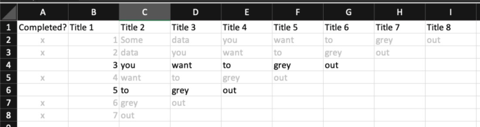
A quick how-to for Excel explaining how to ‘grey out’ an entire row based of value of one cell – in this case each cell with an ‘x’ in column A. I often use this at work to track progress of various spreadsheets for different deployment projects.
I’ve made this ‘How-To’ using Excel on MacOS – some steps might be slightly different on Windows, but same principals and formulas apply.
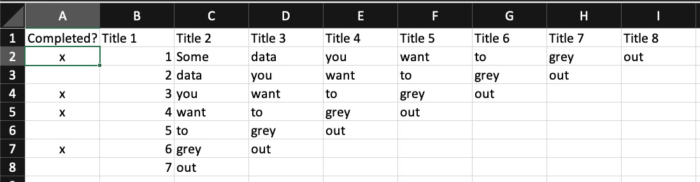
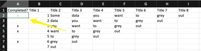
First select any cell in row 2, A2 as an example.
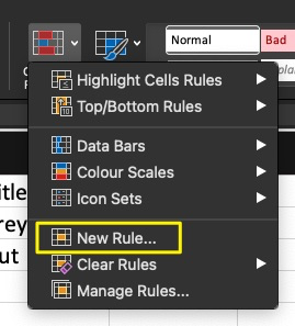
Go to ‘Conditional Formatting‘->’New Rule‘
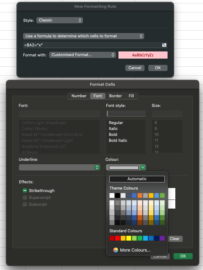
Under ‘Style:‘ select ‘Classic‘ and then ‘Use a formula to determine which cells to format‘
In the formula bar type ‘=$A2=”x”‘ – pay attention to dollar sign. It has to be in the right place for this to work.

Then under ‘Format with:‘ select ‘Customised Format…‘
You can customise it in any way you like. I like to keep it simple and change the colour of the text to grey. It makes rest of the cells stand out. You could add ‘Strikethrough’ effect or change size; or even style of the font on top of changing the colour.
Confirm your customisation options by pressing ‘OK‘ and then ‘OK‘ again on the ‘New Formatting Rule’ window.
You will notice that the new conditional formatting is applied only to the cell you had select. To apply this condition to all rows go to ‘Conditional Formatting‘->’Manage Rules‘ and locate the rule you have just created.

If you are unable to see it, change selection to show formatting for ‘This worksheet‘ instead of ‘Current Selection’.

In the field ‘Applies to‘ type ‘=$1:$10‘, or any number of rows you want to apply this condition to, then press ‘OK‘.

You will now see that all rows with an ‘x‘ in first column are greyed out to mark them as completed.